Model of the Earth's Magnetic Environment (MEME)
Each year BGS produce a ‘parent’ model of the magnetic field termed the 'Model of the Earth's Magnetic Environment' (MEME). This is used for scientific study and is continually improved to accommodate new geophysical understanding and computational techniques. It is used as a basis for a number of models - BGS Global Geomagnetic Model (BGGM), World Magnetic Model (WMM), International Geomagnetic Reference Field (IGRF).
The input data
BGS uses data from magnetic survey satellites, for example Ørsted, CHAMP and the ESA Swarm satellites, and from observatories around the world (including the nine observatories BGS operate). These data are selected for two purposes: (1) to cover the period of time which we want to model the magnetic field and (2) to remove as much noise in the data as possible; for example, by excluding data collected during geomagnetic storms.
The model
MEME captures both the time-varying and the spatially-varying components of the magnetic field. The time variations are modelled with high order B-splines for the internal field and by linear and periodic functions with dependence on magnetic activity for the external field. The spatial variations are modelled using spherical harmonics extending to the maximum degree and order that can be supported globally by the input data.
Capturing the variations in time
The Earth's internal magnetic field is generated by the motion of the conductive metallic fluid in the outer core. Changes in the motion of the fluid cause variations of the shape and intensity of the magnetic field measured at the surface - this change over time is known as secular variation (SV).
However, SV itself is not constant and changes on decadal timescales, with occasional periods of rapid variations in the second time derivative of the field (or secular acceleration (SA)) which are called geomagnetic jerks.
Geomagnetic jerks are most commonly defined as ‘∨’ or ‘∧’ shaped features in the SV as illustrated in Figure 1. The upper panel shows an idealised version of a jerk, while the lower panel shows what they look like in real observatory data, using the 1969 jerk recorded in the East (Y) component at Eskdalemuir.
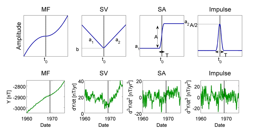
Jerks represent the most rapid observed internally generated magnetic features known and are associated (we think) with fast flows at the surface of the outer core, which can give us clues about the kinds of processes going on in a region we can never visit.
Jerks are still not fully understood, and appear sporadically and apparently randomly in the magnetic field record. Using global models of the magnetic field rather than just single points on the surface can help us understand their source within the outer core and their temporal evolution.
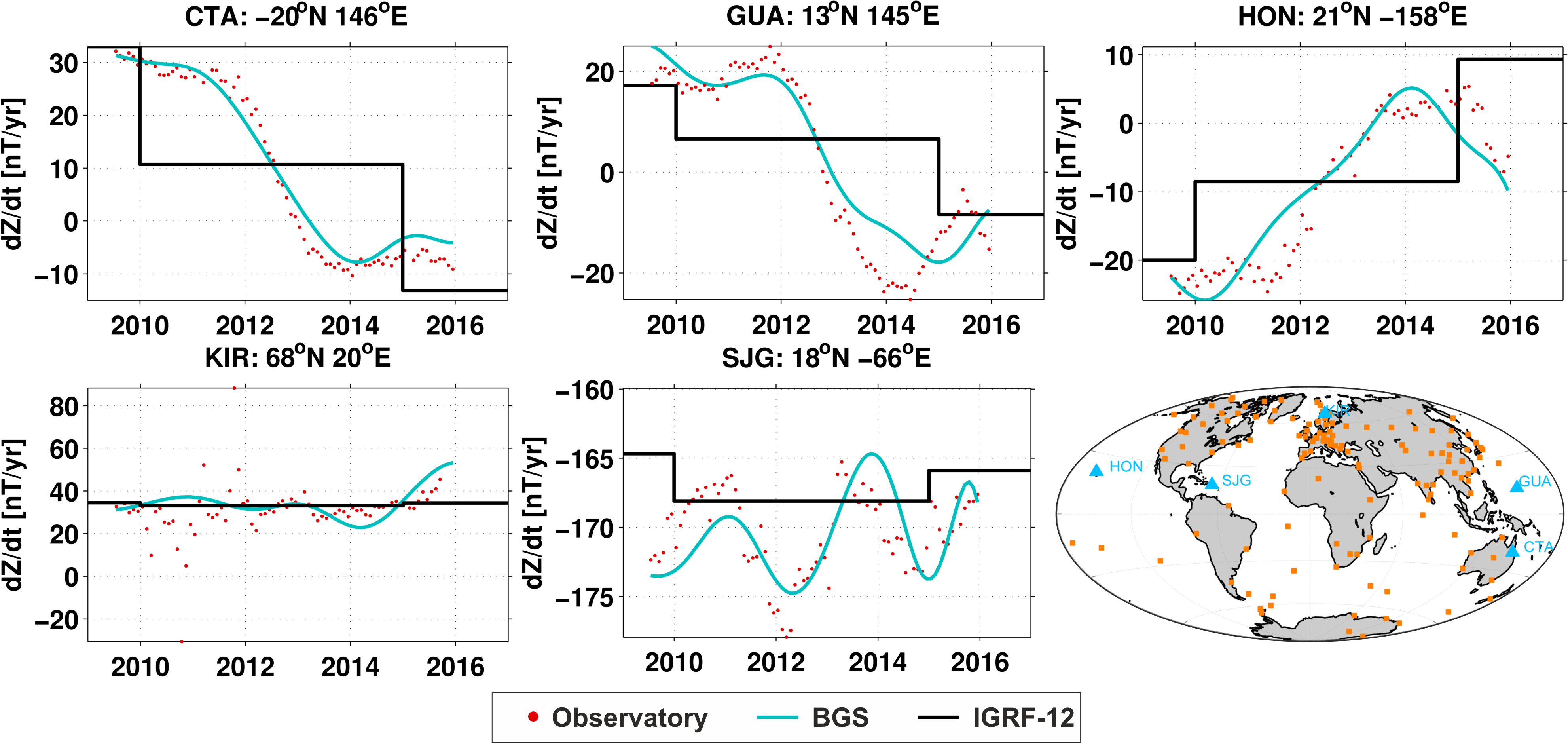
Jerks appear to happen every few years - the most recently accepted jerk was around March 2014 but there may have been a new jerk as recently as June 2015. We have used the MEME2016 model as well as observatory time series to make maps of the jerks. In some places they are negative (i.e. ‘∧’-shaped) and in some areas they are positive (or ‘∨’-shaped). Figure 2 shows the polarity as detected in a selection of ground-based observatories around the globe. The data points show the computed annual change of the field. The solid lines are the estimated change of the magnetic field at the locations, as derived from global models. The blue line is the most recent MEME model which captures both the 2014 jerk and suggests that there was a new jerk starting to occur in 2015.
As can be seen in Figure 2, the changes of the magnetic field can vary substantially from location to location. A jerk can be seen around 2014 at four of the five observatories shown, but Guam (GUA) also shows a jerk in mid-2015, the first ground observations of this feature.
Capturing the variations in space
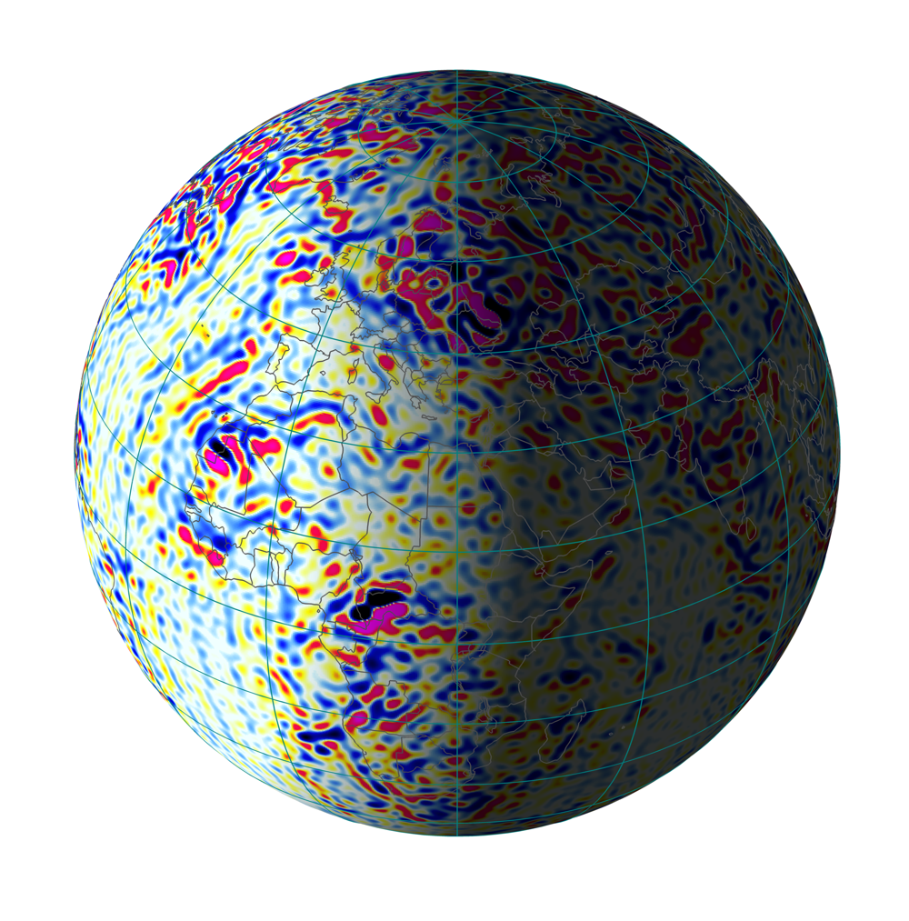
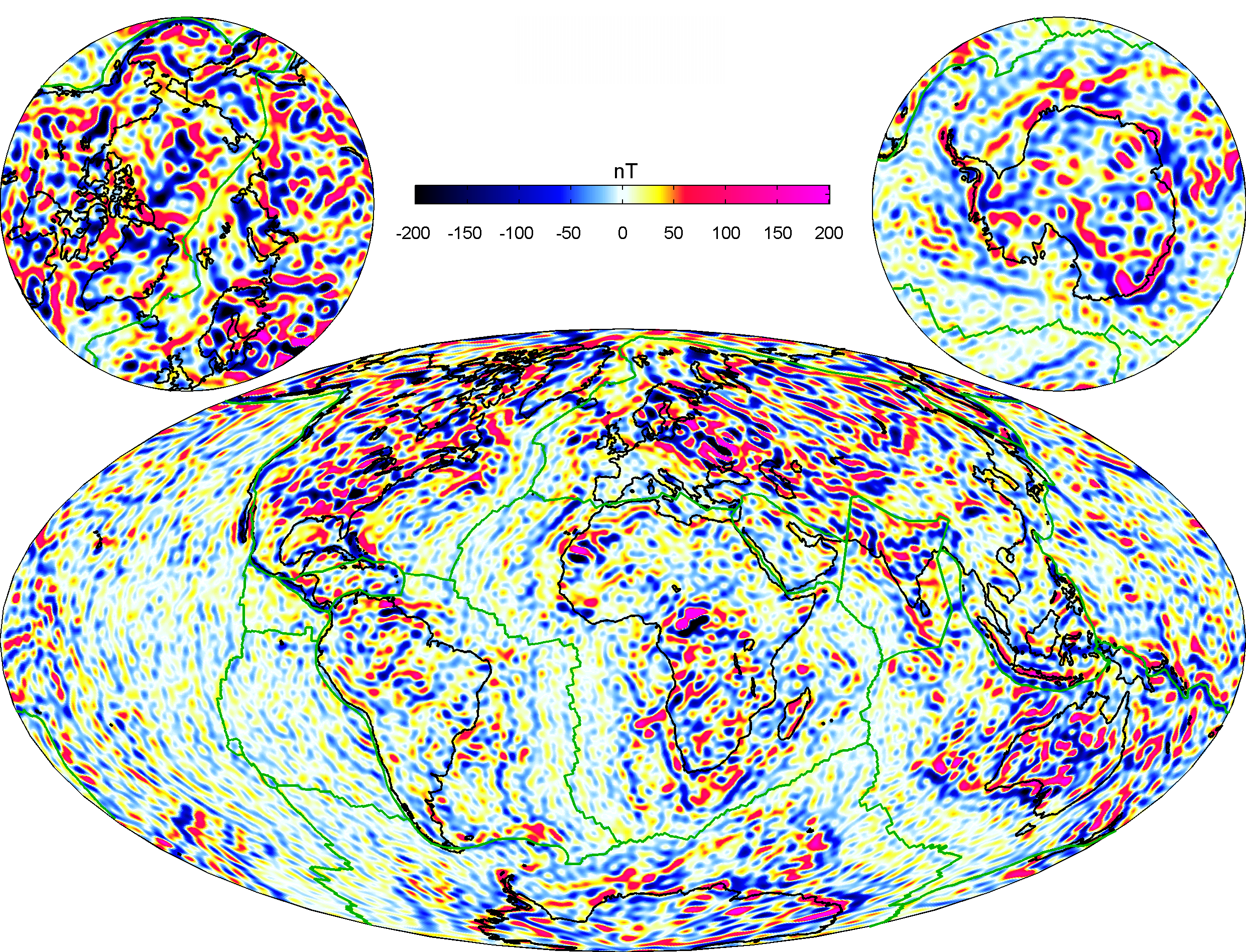
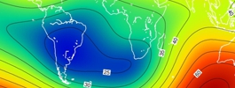
Using the data directly and as gradients we can iteratively solve, with a priori constraints, spherical harmonic coefficients to high degree. The gradient data are derived from satellite measurements, specifically along-track (and cross-track if data from Swarm) low latitude vector data differences and high latitude, linearised scalar data differences. Figure 3 shows the high resolution now possible using these techniques.
References:
- Brown, W., Mound, J. & Livermore, P., (2013). Jerks abound: An analysis of geomagnetic observatory data from 1957 to 2008. Phys. Earth Planet. Inter. 223, 62:76. doi: 10.1016/j.pepi.2013.06.001.
- Brown, W., Beggan, C. & Macmillan, S. (2016). Geomagnetic jerks in the Swarm Era. In ESA Living Planet Symposium Proceedings, Spacebooks Online.
- Thébault, E et al., (2016). International Geomagnetic Reference Field: the 12th generation. Earth Planets Space, 67(79). doi: 10.1186/s40623-015-0228-9.
- Global Geomagnetic Models
- Space Weather and Geomagnetic Hazard
- High-frequency magnetometers
- Schumann Resonances
- Geoelectric field monitoring
- Space Weather Impact on Ground-based Systems (SWIGS)
- SWIMMR Activities in Ground Effects (SAGE)
- Geomagnetic Virtual Observatories
- Quantum magnetometers for space weather
- Magnetotellurics
- Publications List
