Improving our predictions of secular variation using estimates of flows of molten material in the Earth's core
Secular variation (SV) is typically defined as the slow annual to decadal change of the Earth�s magnetic field and is caused by the flow of liquid in the outer core, deep inside the Earth. The change of the field is not easily predictable due to the nature of the flow regime in the core and the mechanism by which the magnetic field is generated. However, an estimate of the instantaneous flow itself can be computed, if we make some assumptions about its nature and how it affects the magnetic field we observe at the surface. If we have a longer series of data we can compute the accelerated flow too.
Researchers usually assume that the magnetic field is effectively ‘frozen’ into the liquid under the surface of the core-mantle boundary (approximately 3000 km below the Earth�s surface). This means the magnetic field is advected by the flowing liquid (i.e. drifts along with it) over short timescales (< 10 years, say). In reality, the actual interaction between the liquid in the outer core and the magnetic field is far more complex and is currently poorly understood in detail. However, if the simplifying assumption is made that any observed change in the spatial pattern of the magnetic field is due to fluid flow, we can mathematically ‘invert’ the changes in the magnetic field we measure at and close to the surface of the planet to infer the pattern of fluid flow at the top of the outer core.
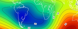
Using several years of magnetic field observations from observatories and satellites can help us build up a picture of what the large-scale flow patterns in the core look like (this is known as a �steady flow model�). Figure 1 (top) shows an image of the changes of the magnetic field and the flow patterns that could cause this on the core-mantle boundary (continents shown for reference). In the Atlantic hemisphere, the flow tends to be relatively fast, while in the Pacific hemisphere it is slow or non-existent. The change of the magnetic field variation and hence the accelerated flow is about ten times smaller (bottom). This map also shows strong changes in the Indian Ocean, suggesting this is a location of relatively rapid acceleration.
![Figure 1: [Left] Downward component (Z) of the global magnetic field SV and acceleration. [Right] Steady flow and acceleration models at the core-mantle boundary for 2010.0 (continents shown for reference).](Fig1_SV_SA_FlowAcc.png)
In a manner analogous to weather forecasting, we can imagine that this flow pattern �pushes� (or advects) the magnetic field with it, should it continue to flow in this manner for several years. We can now use the flow and acceleration models to forecast the change in the magnetic field over a short period (2-5 years).
Testing the flow models against IGRF-11 predictions
The IGRF and WMM magnetic field models provide estimates of the average SV (annual change) of the field expected over the five years following on from their release date. The estimates are mainly based upon linear extrapolation of the magnetic field from the observed change in the previous few years. However, the estimate is often relatively inaccurate at the end of the five-year forecast period. Can the forecasts from core flow models better predict the SV over five years? We can test this by comparing the models directly and to independent observatory data collected on the ground.
We compared the forecast from the BGS flow forecast from 2013 to the forecast from the 11th version of the International Geomagnetic Reference Field (IGRF) released in December 2009 (Finlay et al., 2010). This is not an entirely fair comparison as the IGRF model is only updated every five years, compared to the annual update of the BGS model, so we note the differences are more illustrative of the variation of the magnetic field and our current ability to predict it than a critique of the IGRF-11.
Figure 2 shows the spatial difference in the three components (North [X], East [Y] and Down [Z]) of the magnetic field between the prediction of IGRF-11 and the BGS magnetic field model of 2013, plus the projection forwards over two further years until 2015. The bulk of the magnetic field data for the BGS model comes from the CHAMP satellite prior to 2011.0.
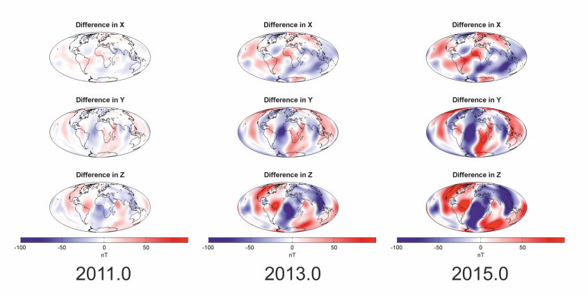
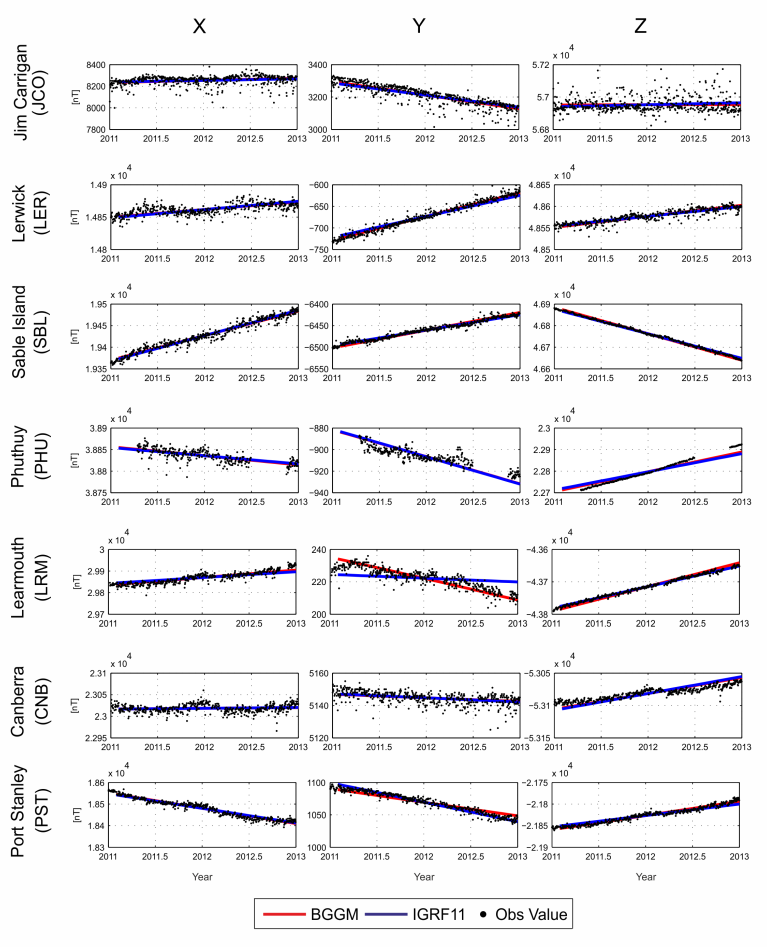
Figure 3 shows the predicted values of the magnetic field at seven globally distributed observatories across the world. The dots are the hourly-mean values during local time 02:00-03:00 when it is magnetically quiet at each observatory. The blue line shows the forecast IGRF values for each component and the red line shows the BGS flow model forecast. Note that the red and blue lines have had the mean crustal bias in each component at each observatory removed in order to show how the difference from the observatory data varies with time. Figure 3 shows that the forecast from both models is reasonably good but, overall, the BGS achieves better results due to having additional data up to 2011.0 and through using the flow forecast method.
The use of flow modelling to provide a more physics-based method improves the prediction of magnetic field change compared to simpler extrapolation methods. Further details can be found in Beggan and Whaler (2010) and Beggan et al. (2014).
References
Beggan, C. and Whaler, K. (2010), Forecasting secular variation using core flows, Earth Planets Space, 62 (10), 821-828, doi:10.5047/eps.2010.07.004
Finlay, C.C., Maus, S., Beggan, C.D., Hamoudi, M., Lowes, F.J., Olsen, N., Thebault, E., (2010). Evaluation of candidate geomagnetic field models for IGRF-11. Earth Planets and Space, 62 (10). 787-804. doi:10.5047/eps.2010.11.005.
- Global Geomagnetic Models
- Space Weather and Geomagnetic Hazard
- High-frequency magnetometers
- Schumann Resonances
- Geoelectric field monitoring
- Space Weather Impact on Ground-based Systems (SWIGS)
- SWIMMR Activities in Ground Effects (SAGE)
- Geomagnetic Virtual Observatories
- Quantum magnetometers for space weather
- Magnetotellurics
- Publications List
